The Anatomy of Machine Learning: Data, Models, Loss, and Optimization

A program that converts Celsius to Fahrenheit is written by hand: someone knows the rule, $f(x)=1.8x+32$, and types it. Machine learning starts from the other end. We have pairs $(x,y)$, measurements with some noise, and no rule. Learning means choosing, from a family of candidate functions, the one whose predictions stay closest to $y$, and hoping it also works on pairs we have not seen yet.

Everything below is one piece of that sentence: the pairs (data), the family (model), "closest" (loss), "choosing" (optimization), and "pairs we have not seen" (generalization).

The setup

We assume the examples come from an unknown distribution $P_{\text{data}}(x,y)$. We never see that distribution, only a finite dataset $\mathcal{D}=\{(x^{(i)},y^{(i)}){\}}_{i=1}^N$ drawn from it.

The model defines a hypothesis space $\mathcal{H}$: all the functions $h_{\theta }$ it can represent as its parameters $\theta$ vary. What we want is the $h_{\theta }$ with the smallest error on new samples from $P_{\text{data}}$. We cannot measure that directly, so we minimize the average error on $\mathcal{D}$ and check the result on data kept aside.

Four components

Forward pass and loss evaluation against the targets

Model capacity and inductive bias

The model decides which shapes of function can be learned at all. A linear model can only represent straight lines (hyperplanes in higher dimensions): a strong inductive bias, an assumption built in before seeing any data. A deep neural network can represent far more complex functions, and its biases come from its architecture: a convolutional network, for instance, assumes that nearby pixels are related.

How flexible the family is, is the model's capacity.

The bias-variance tradeoff

• Too little capacity (high bias): the model cannot capture the structure in the data. It underfits: errors are high on the training set and on new data.
• Too much unchecked capacity (high variance): the model fits the noise along with the signal. It overfits: low training error, high error on new data.

Underfitting, a good fit, and overfitting

Measuring error: the loss

The loss turns "how wrong" into a single number $\mathcal{J}(\theta )$. Two common choices:

• Regression, mean squared error: $\mathcal{J}(\theta )=\frac{1}{N}{\sum }_{i=1}^N(y^{(i)}-{\hat{y}}^{(i)}{)}^2$
• Classification over K classes, cross-entropy: $\mathcal{J}(\theta )=-\frac{1}{N}{\sum }_{i=1}^N{\sum }_{k=1}^K{y}_k^{(i)}\log {\hat{y}}_k^{(i)}$, where $y^{(i)}$ is the one-hot label and ${\hat{y}}^{(i)}$ the predicted probabilities. Only the probability given to the correct class counts, and the loss grows quickly as that probability approaches 0.

Training looks for the parameters that make the loss smallest:

The training loop

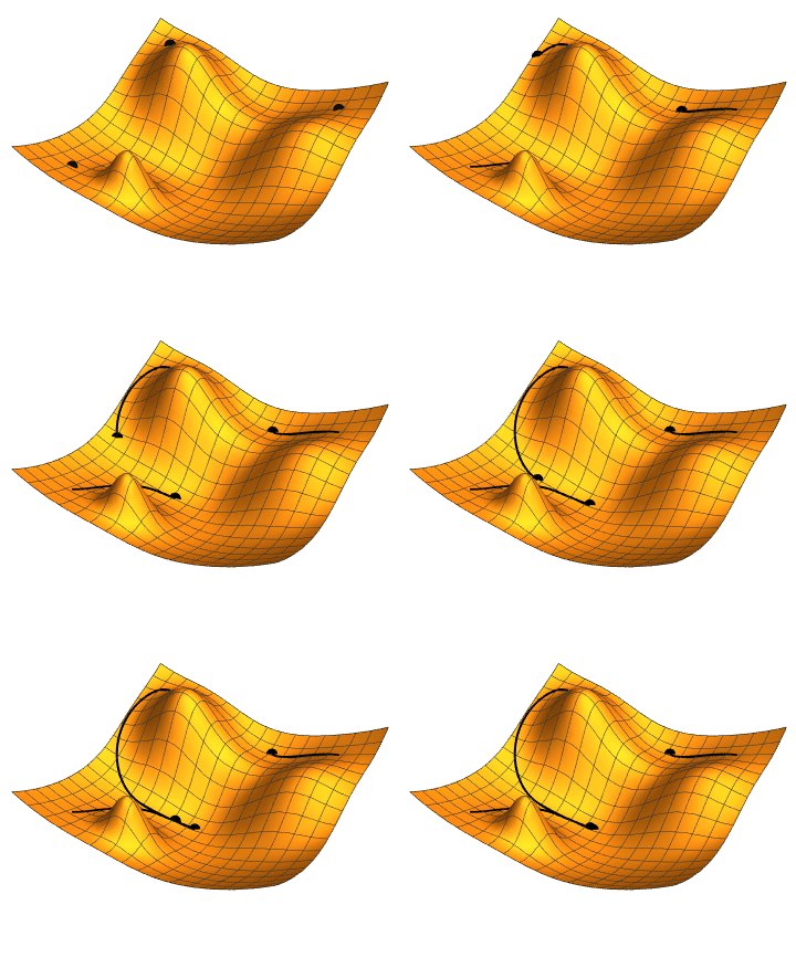
For neural networks, the minimum is found step by step: compute the gradient of the loss, the direction in which it increases fastest, and move the parameters a little in the opposite direction. How long each step should be is a question of its own, covered in the article on gradient descent and step size (in French).

The full training loop

1. Forward pass

   Pass a batch of inputs $x$ through the model $h_{\theta }(x)$ to get predictions $\hat{y}$.

2. Loss computation

   Compare the predictions $\hat{y}$ with the targets $y$ through the loss $\mathcal{J}(\theta )$.

3. Backward pass (backpropagation)

   Compute the gradient of the loss with respect to every parameter, using the chain rule: ${\nabla }_{\theta }\mathcal{J}(\theta )$.

4. Update

   Move the parameters against the gradient, scaled by the learning rate $\eta$:

   $${\theta }_{\text{new}}={\theta }_{\text{old}}-\eta \cdot {\nabla }_{\theta }\mathcal{J}(\theta )$$

Gradient descent on a two-parameter loss surfaceJacopo Bertolotti, Wikimedia Commons, CC0

A minimal implementation in PyTorch

The Celsius idea, with a different rule: data generated from $y=2x+1$ plus noise, and a linear model that has to find the two numbers back.

# train_regression.py
import torch
import torch.nn as nn
import torch.optim as optim
 
# 1. Synthetic data: y = 2x + 1, plus noise with standard deviation 0.1
torch.manual_seed(42)
X = torch.randn(100, 1)
y = 2.0 * X + 1.0 + 0.1 * torch.randn(100, 1)
 
# 2. Model: one weight and one bias
model = nn.Linear(in_features=1, out_features=1)
 
# 3. Loss and optimizer
criterion = nn.MSELoss()
optimizer = optim.SGD(model.parameters(), lr=0.1)
 
# 4. Training loop
for epoch in range(101):
    y_pred = model(X)
    loss = criterion(y_pred, y)
 
    optimizer.zero_grad()
    loss.backward()
    optimizer.step()
 
    if epoch % 25 == 0:
        print(f"Epoch {epoch:03d} | Loss: {loss.item():.4f}")
 
w, b = model.weight.item(), model.bias.item()
print(f"Learned: y = {w:.2f}x + {b:.2f}")

Each step here uses all 100 examples, so optim.SGD is doing plain (full-batch) gradient descent; the "stochastic" part appears when each step sees only a random batch.

Two things about the output can be predicted without running it. The noise has a standard deviation of 0.1, so no straight line can reach a mean squared error much below $0.1^2=0.01$ on this data: the printed loss should fall and level off near that value. And the learned line should be close to $y=2x+1$. The exact printed numbers depend on the PyTorch version and the random initialization, so they are not reproduced here.

Generalization and the held-out split

An example split: 70% training, 15% validation, 15% test

What matters is performance on data the model has never seen. The training set is used to fit the parameters, the validation set to choose between models and settings (capacity, learning rate, when to stop), and the test set is used once, at the end, to estimate how the chosen model will do on new data. The 70/15/15 proportions are a convention, not a rule; with little data, cross-validation reuses it more efficiently.

References

1. Zhang, C., Bengio, S., Hardt, M., Recht, B., & Vinyals, O. (2017). Understanding Deep Learning Requires Rethinking Generalization. ICLR 2017.
2. Keskar, N. S., Mudigere, D., Nocedal, J., Smelyanskiy, M., & Tang, P. T. P. (2017). On Large-Batch Training for Deep Learning: Generalization Gap and Sharp Minima. ICLR 2017.
3. Dinh, L., Pascanu, R., Bengio, S., & Bengio, Y. (2017). Sharp Minima Can Generalize For Deep Nets. arXiv:1703.04933.